
PROMOT Computer Program
PROMOT (PRObe vehicle concept for MOnitoring
road Traffic) studies the efficiency of the probe vehicle concept in general and
the compares the performance protocols for uplink probe vehicle transmission, viz. ALOHA and polling. To a limited extent, it can be used a
network planning tool.
 Promot runs under DOS, and has a menu structure to enter parameter of the calculations or simulation. It is located at
software/ivhsprog.zip.
Brief instructions for installation are available.
Disclaimer: The software has no guarantee of any type whatsoever.
The user agrees that neither the publisher nor the editor / authors
will be held liable for any damages, including lost profits, savings, or any
incidental or consequential damages arising out of the use or presence
of any program.
The PROMOT Model
A model covering road traffic aspects as well as data communication aspects, has
been developed in order to implement a performance analysis of obtaining real-time road
traffic
data from probe vehicles through a mobile communication infrastructure. This multi-disciplinary
model has been
called PROMOT (PRObe vehicle concept for MOnitoring road Traffic) and consists of
several sub-models.
Road and Public Transport Network Specification (sub-models 1 and 2)
The starting point of the PROMOT model is a network sub-model of the transportation
infrastructure. For reasons explained in the concerning (sub-)section the inter-urban network
specification includes private as well as public transport while the urban network specification
is
limited to private transport only. Nodes (concentrations of population and employment) and
connecting links (roads and rail with specific capacities) are used.
Transportation Model (sub-models 3 through 7)
The origin-destination (O-D) matrix is an essential component for computing road traffic
flows.
It specifies the number of vehicles coming from and heading to the different network nodes.
For
the inter-urban traffic flow computation a measured OD-matrix for peak hour traffic was not
available for this study, so we estimated one by means of this Transportation Model. To this
end, we modified an existing model of combined multi-modal static interaction and applied
elastic land-use constraints. This model calculates the number of departures and arrivals (trip ends)
of
each specified zone. It assumes accessibility to be the main factor influencing land-use. The
model is an extension of the traditional four-stage transportation model which is a step-wise
approach to production/attraction, distribution, mode choice, and assignment.
In our case however, the distribution and mode choice are calculated
simultaneously. It uses elastic, rather than fixed constraints. In this way, the land-use data
(employment and working population) that are traditionally exogenous in a fixed constrained
interaction model, are computed endogenously.
Sub-model 3 computes the number of trip ends in each zone from the employment and
working
population using several trip purposes. The generalized time (which expresses an average of
different sacrifices needed for traveling, such as travel time and costs, expressed in units of
time) is calculated for trips between origin-destination pairs, both for the road travel (sub-
model
4) and for the public transport (sub-model 5). Based on these generalized times, sub-model 6
computes and sub-model 7 distributes the trip ends over the network along the shortest
routes
between every zone. Traffic measurements have been used for verification of the resulting
O-D
matrixes.
Traffic Assignment (sub-models 8 and 9)
The former computations result in an origin/destination (OD)-matrix for car trips (and in the
case of the inter-urban area traffic flow computation also for public transport trips). In sub-
model 8, the road OD-matrix is assigned to the road network. This results in traffic flows on
each road link. The transportation model thus provides the traffic flow and mean travel time
for
each road link (sub-model 9).
Generation of Traffic Messages (sub-models 10 and 11)
A certain percentage of the vehicles serves as probes that transmit traffic messages. Sub-
model
11 determines the number of probe vehicles on a road link directly from the computed traffic
densities on each road link. Alternatively, in sub-model 10, we simulate each probe vehicle
traveling from its origin to its destination. In both cases, we assume that a probe vehicle
transmits its location and its travel time over the last (fraction of a) road link. The optimal
content and data format of the traffic messages is still a subject for investigation. We assume
that vehicles perfectly know their location, for instance through a hybrid GPS and dead-
reckoning positioning technique.
Calculation of Spatial Throughput (sub-models 12, 13 and 14)
The traffic messages can be received by base stations located in the area under study. In the
supply communication network, harmful interference between messages transmitted in the
same
time slot (collisions) may occur. Message collisions are taken into
account
using models for receiver capture and mobile radio wave propagation (sub-model 12 for the
simulation and sub-model 13 for the analysis).
Performance of ATMS/ATIS Services
(this is not a PROMOT sub-model)
The final result of the PROMOT computations is an overview of the number of received
traffic
messages (throughput) and their locations. A further crucial aspect of probe vehicle data collection is to
relate
this number of received probe vehicle messages to the
number of probe messages needed
to perform several ATMS and ATIS services.
Network Specification
An infrastructure network incorporates at least two elements, namely links and connecting
points. The purpose of links is to concentrate flows of traffic so that a collective infrastructure
can be constructed. The connecting points are represented by nodes which connect
(dis)similar
links and where a network can be entered or left.
At the highest functional level of abstraction of road traffic infrastructure we find the inter-
urban
roads, such as interstates, express ways and freeways, with the principal objective to connect
different areas of community. With respect to their shape inter-urban roads can be classified
into
five distinct base types, namely: linear or
axial,
star shaped or radial, circular, rectangular or grid and triangular. With
respect
to their location in relation to urban agglomerations tangential and radial inter-urban roads
can
be distinguished. The inter-urban road network in the Netherlands is characterized by a
tangential location and a triangular shape. The inter-urban road network in the USA has a
grid
structure and also a tangential location in relation to urban agglomerations. At a lower
functional level of abstraction of road traffic infrastructure we find the urban roads, such as
highways, motorways and highstreets, with the principal objective to facilitate the different
parts
of the urban area. In essence three distinct base types of urban roads can be distinguished,
namely: linear or axial, star shaped or radial, and rectangular or grid structure. In particular
because urban areas in the Netherlands have generally originated and urban areas in the
USA
have usually been constructed, Dutch urban road networks are mostly characterized by a
circular or radial shape (organic structure), while American urban road networks are mostly
characterized by a grid structure.
It is generally recognized that the effectiveness of mobile data
protocols depends
among other things the number of mobile transmitters, the temporal distribution of mobile
transmitters, and the spatial distribution of mobile transmitters. Hence, it can be envisaged
that
in urban area road networks, with relatively low traffic flows and speeds, and in inter-urban
area road networks, with relatively high traffic flows and speeds, the behaviour of the probe
vehicle concept will differ. For these reasons, two different types of road networks have been
selected in the Network Specification Model (sub-models 1 and 2) to analyze the
performance
of the probe vehicle concept and to use within the PROMOT model.
 The first one is an inter-
urban area road network with a grid structure and a tangential orientation, namely the
freeway
network in the San Francisco Bay Area.
The first one is an inter-
urban area road network with a grid structure and a tangential orientation, namely the
freeway
network in the San Francisco Bay Area.
The second one is an urban area road network with
a
ring-shaped structure and a radial orientation, namely the motorway and highstreet network
of
Eindhoven.
Each link in the network specification (both inter-urban and urban) contains the following
attributes:
- - begin node (A-node),
- - end node (B-node),
- - capacity,
- - speed in unloaded condition, and
- - one-way or two-way road.
Inter-Urban Road Network
For the inter-urban network specification, we took the San Francisco Bay Area (San
Francisco-
Oakland-San Jose). This area was divided into network nodes representing zones with the
most
important attributes `dwelling' and `employment'. These nodes are connected by links,
representing the road infrastructure. Each trip starts and ends in a certain node.
This Figure shows the abstracted road network of the San Francisco Bay Area. This
abstracted
network has been limited to the major roads (mostly highways) and comprises 40 zones and
63
links. In order to be able to apply the Transportation Model also the
major public transport lines in the San Francisco Bay Area have been added (17 nodes and
17
zones). For trips by public transport the speed outside the public transport
network has been taken high (15 km/h), assuming that the car will be used in pre- and post-
transport.
Urban Road Network
Monitoring a complete urban area road network by means of infrastructure based traffic
detectors would require an immense amount of such traffic detectors due to the small-scale
lay-
out of such a network, with many short road links and many crossroads, and is therefore
hardly
possible. A monitoring system with roving probe vehicles
would seem more appropriate under these conditions. In order to analyze the performance of
the
probe vehicle concept in an urban area also an urban area traffic flow computation has been
performed. The urban area performance analysis should not only express exterior contrasts,
such as differences in shape and traffic load of inter-urban and urban road networks, but also
interior differences. The urban area network specification should therefore also consider
several
types of roads, ranging from small, lightly loaded to large, heavily loaded roads. In particular,
the combination of several distinct types of roads is important to investigate whether or not
the
smaller roads are predominated by the larger roads. For this reason the highways around the
city of Eindhoven, the entrance and exit roads to and from the city of Eindhoven, the ring
road
in Eindhoven as well as the lower class roads have been selected for the urban network
specification.
The network specification of the urban area of Eindhoven is based on data from the Dutch
Rijkswaterstaat and the municipality of Eindhoven. This data has been
aggregated
into a road network of 81 nodes and 266 links. This data was
sufficiently comprehensive to perform a traffic flow computation for the urban area of
Eindhoven and therefore a public transport network specification was not required.
Transportation Model
Most existent transportation models can be brought back to the general structure of the
classic
four-stage transportation model. Although the classic model is presented as a sequence of
four
sub-models, it is generally recognised that the process of traveling does not actually take
place
in this type of sequence.
Socio-economic data is "used to estimate a model of the total number of trips generated and
attracted
by each zone of the study area (trip generation). The next step is the allocation of these trips
to
particular destinations, in other words their distribution over space, thus producing a trip
matrix. The following stage normally involves modeling the choice of mode and this results in
modal split, i.e. the allocation of trips in the matrix to different modes. Finally, the last stage
in
the classic transportation model requires assignment of the trips by each mode to their
corresponding network: typically private and public transport.".
For the urban traffic flow computation all required travel and traffic data was available to
perform each of the above-mentioned steps.
For the inter-urban traffic flow computation straight-forward execution of the above-
mentioned
steps was not possible as accurate data about trip generation was not available. For this
reason a
divergent Transportation Model, which integrates the first three steps of the classic
transportation model, has been used to compute this trip generation data from available, but
much more global, data.
Inter-Urban Road Network
The theoretical foundation for the Transportation Model is a micro-economic theory under
money and time constraints, stating that each
persons maximizes the difference between utility of where he/she lives and works and the
sacrifice (generalized time, which expresses an average of different sacrifices needed for
traveling, such as travel time and costs, expressed in units of time) of the commute.
The Transportation Model computes the trip generation, that is
the
number of departures and arrivals (trip ends) of each network zone, assuming accessibility to
be
the main factor influencing the process of trip generation. Therefore, the components
distribution and modal split are calculated simultaneously and elastic, rather than fixed
constraints are used. In this way, the land-use or trip generation data (defined as
employment
and working population) that are traditionally exogenous in a fixed constrained interaction
model, are computed endogenously.
Urban Road Network
For the urban traffic flow computation measured data was available (from the MER/trace
study
into construction of the motorway A50. Because the area subdivision in both
studies slightly differed, the available data had to be adapted to fit the specified urban road
network of Eindhoven. Subsequently, the same distribution computations were performed as
described in the previous sub-section (the available data concerned road traffic only and
therefore the modal split could be omitted).
Inter-Urban Road Network
Figure 5.6 illustrates the road traffic flows during the evening rush hour on the inter-urban
freeway network of the San Francisco Bay Area, found according to the assignment scheme
discussed above. The thickness of the links indicates the size of the traffic flow qa. The
different
hatches of the links represent qa / ca, i.e., the amount of vehicle traffic traveling on the road
link relative to the capacity of that link and provide estimates of link travel times. A ratio of
qa /
ca is 0.85 or higher indicates congested traffic.
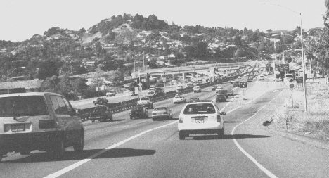
PROMOT Screen Dump: Intensity of messages transmitted by probe vehicles in San Francisco Bay Area.
Penetration 1%, one transmission per probe vehicle every 60 sec.
Figure 5.6 Computed road traffic flows during the evening rush hour
on the inter-urban freeway network of the San Francisco Bay Area
Detailed validation of the estimated road link flows with real traffic measurements could not
be
done as no accurate data was available. Rough comparison with the traffic situation on the
freeways in the San Francisco Bay Area during average peak hours indicated that the
estimations are realistic. For our purpose, i.e., creating a sufficiently realistic traffic situation
to
evaluate the performance of the probe vehicle concept for collecting traffic messages in an
inter-
urban road network, this verification is believed to be adequate, as it pictures an average
traffic
situation in the Bay Area.
Urban Road Network
The road traffic flows are computed for the evening rush hour on the
urban
road network of the city of Eindhoven, and are found according to the assignment scheme discussed
above. Again, the thickness of the links indicates the size of the traffic flow q_a, and the
different
hatches represent q_a / c_a, i.e., the amount of vehicle traffic traveling on a road link relative to
the capacity of that link and provide estimates of link travel times. A ratio of q_a / c_a of 0.85 or
higher indicates congested traffic.
Generation of Traffic Messages
In sub-models 10 (analysis) and 11 (simulation), the fleet of probe vehicles is taken as a
certain
percentage of all vehicles. Probes are assumed to be equipped with
positioning and radio communication equipment. By means of simulation or computation, the
effectiveness of the probe vehicle concept is analyzed. The probe vehicles are
assumed to generate traffic messages according to the supply or the demand transmission
scheme. The transmitted probe messages contain the position of the probe vehicle and the
link
travel time experienced. The process of generating traffic messages under the demand
scheme is
rather straightforward. The base station transmits a polling message to one specific probe
vehicle in its cell and this probe vehicle responds by transmitting its traffic message.
The method to compute the probability of successful transmission is discussed in
a separate text in PDF format.
When
the
probe report is successfully received (unsuccessful reception may occur due to path loss, fading or
noise) the base station polls the probe vehicle next in turn. Whenever the
transmitted
probe report is not successfully received, the base stations re-polls the same probe vehicle
and
may repeat this process a limited number of times before the base station proceeds with the
next
probe vehicle.
Under the supply scheme, the process of transmitting probe vehicles messages is even more
simple as the probe vehicles are assumed to randomly generate traffic messages, without
polling
messages from the base station and actually without coordination between transmission from
other probe vehicles. As a result, mutual interference between messages transmitted from
different probes can occur. Messages transmitted in the vicinity of a base station are more
likely
to capture its receiver than other messages. To study this, the effect of distance on the
distribution of traffic messages received by a listening base station is obtained by simulation
or by numerical evaluation of an analytical model.
Simulation
The simulation generates probe vehicles sequentially, and it follows probes driving along the
calculated shortest routes from their specific origin to their specific destination. Each probe
transmits on average once every T seconds, choosing a random time slot. For every
transmitted
message we store its time slot and, after all probes have been generated and have reached
their
destinations, the data base with time stamps is sorted on time slot (i.e., a chronological
database
results containing all transmitted probe messages). Subsequently for each transmitted
message,
its (area-mean) received power is calculated from a path loss model, as well as the (area-
mean)
interference power from other messages in the same time slot. To include the effect of
fading, a
random experiment decides whether the message is received successfully at a base station.
The
probability of successful reception is in agreement with theoretical models to be described in
the
next section. This process is repeated for all base stations.
The Promot Menus


 .
.
